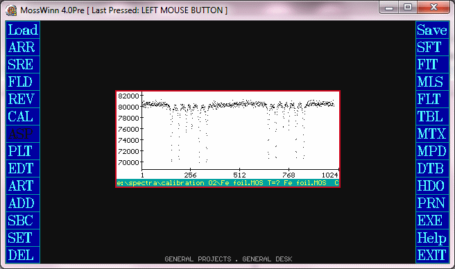
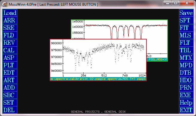
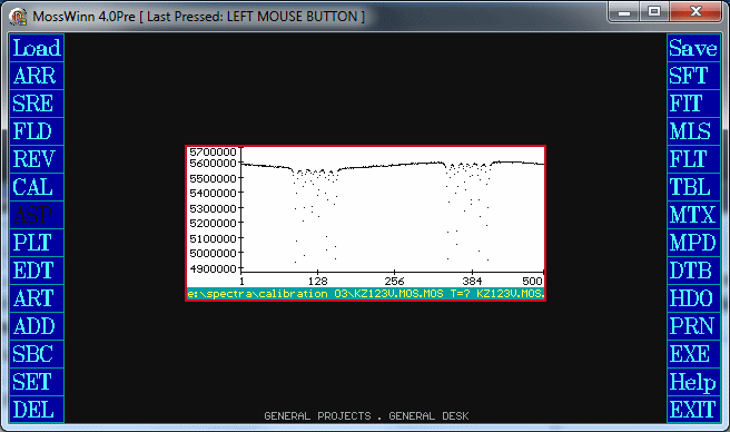
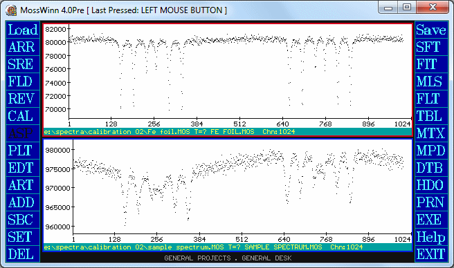
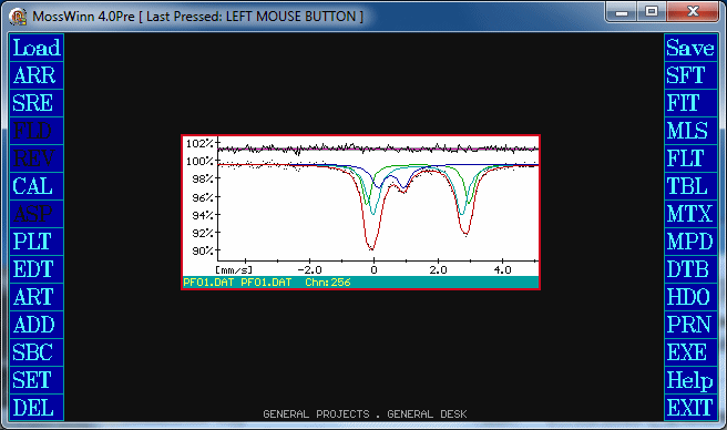
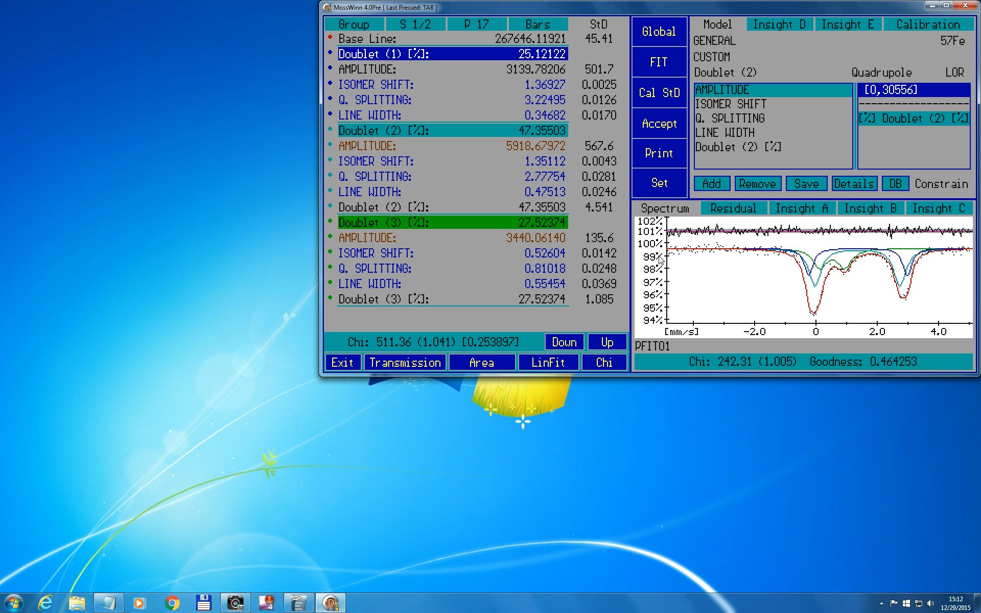
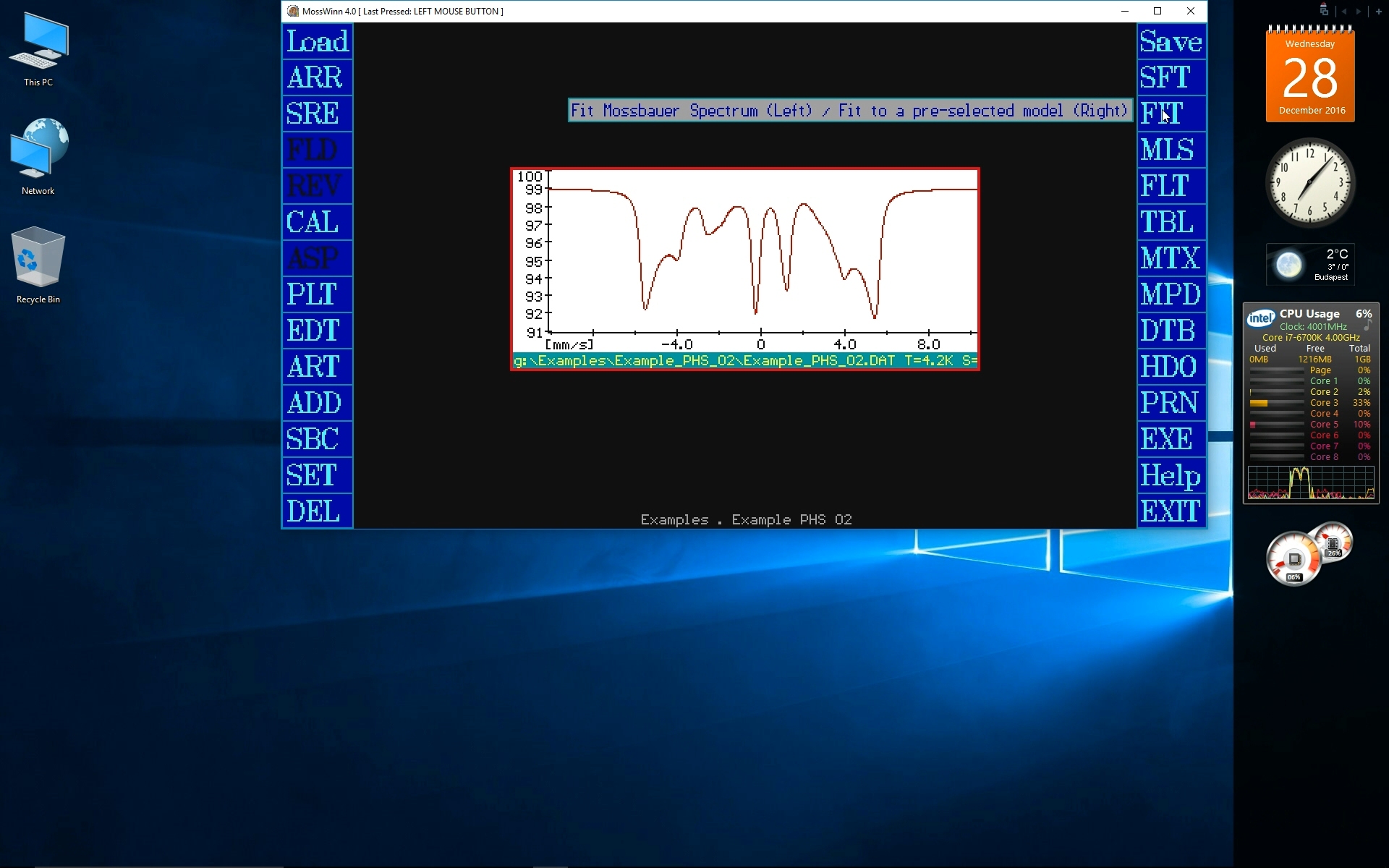
- How to calibrate the velocity axis of a pristine calibration spectrum of α-Fe foil? Follow this tutorial if you intend to calibrate the velocity axis of 57Fe Mossbauer spectra.
- The contribution of the Mössbauer Effect Data Center to the preparation of the Chinese version of the video is duly acknowledged.
|
 Chinese |
 English |
 Without narration |
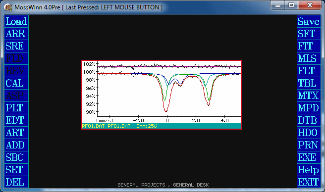
- How to transfer calibration information to a pristine 57Fe Mossbauer spectrum, and how to fit the spectrum to 1 doublet + 1 sextet with constrained line widths?
- The contribution of the Mössbauer Effect Data Center to the preparation of the Chinese version of the video is duly acknowledged.
|
 Chinese |
 English |
 Without narration |
- How to calibrate the velocity axis of a pristine calibration spectrum of α-Fe foil? Follow this tutorial if you intend to calibrate the velocity axis according to the actual velocity of the source in the laboratory frame, such as one would do when calibrating the velocity axis of Mossbauer spectra measured by means of nuclides other than 57Fe. The resulting isomer shifts will then be relative to the source material in this case.
|
 Without narration |
|
|
- How to transfer the previously obtained velocity axis calibration information to a pristine 151Eu Mossbauer spectrum, and how to fit the spectrum to 2 singlets as a first approximation?
|
 Without narration |
|
|
- How to calibrate and fit Mossbauer spectra in their original unfolded state?
|
 Without narration |
|
|
- How to fit 57Fe hyperfine magnetic field distribution with linear correlation between the isomer shift and the hyperfine magnetic field?
|
 Without narration |
|
|
- How to fit a 57Fe magnetic sextet with the 3-4, 2-5 and 1-6 line pairs having independent areas/amplitudes and line widths? This tutorial also shows how to save and reuse a custom subspectrum model set up by the user. Note that in this example the isomer shift is meant relative to that of the 57Co(Rh) source.
|
 Without narration |
|
|
- How to fit the relative areas/amplitudes of the 1-6 and 2-5 lines of a 57Fe magnetic sextet with respect to that of the 3-4 lines? This tutorial makes use of the custom sextet subspectrum model prepared in the previous one. Note that in these examples the fit mode is set to "Area", and consequently the amplitude type parameters give the area of the corresponding individual peaks.
|
 Without narration |
|
|
- This example shows how to set up and save 57Fe quadrupole doublet subspectrum models with parameter boundaries customized for Fe(II) high-spin and Fe(III) high-spin states. The newly created models are then used to fit a spectrum with one Fe(III) and two Fe(II) subcomponents.
|
 Without narration |
|
|
- This example uses the result of the previous one, and shows how to modify the previous model in order to fit the relative area fraction of subcomponents. In addition, it shows how to find an alternative solution to the previous fit problem by assuming that the relative area fraction of one of the Fe(II) components is equal to that of the Fe(III) component.
|
 Without narration |
|
|
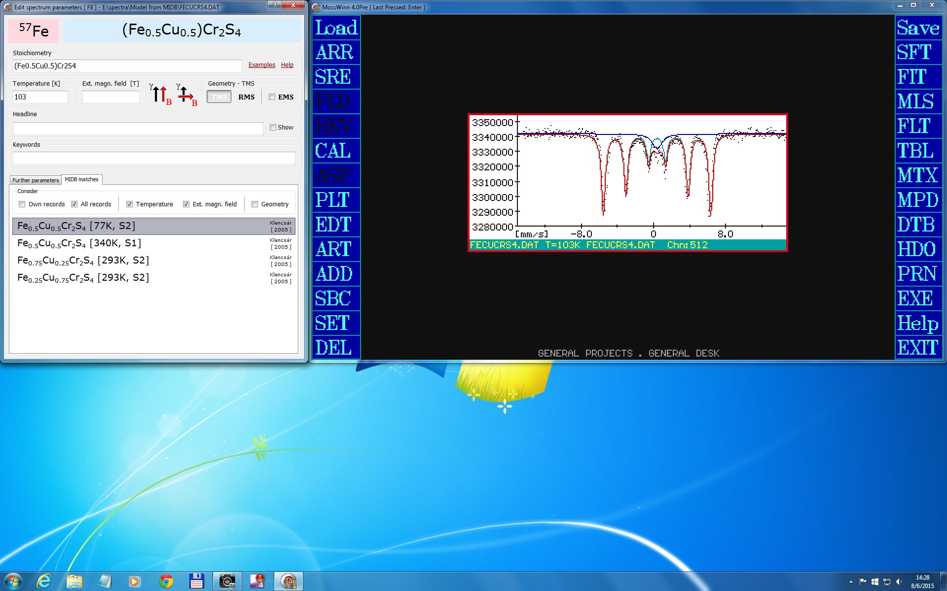
- This example shows how to use the EDT menu for finding in the MIDB database a suitable initial fit model on the basis of the stoichiometry of the measured sample, and how to accept and then fine tune the initial model for a pristine 57Fe Mossbauer spectrum.
|
 Without narration |
|
|
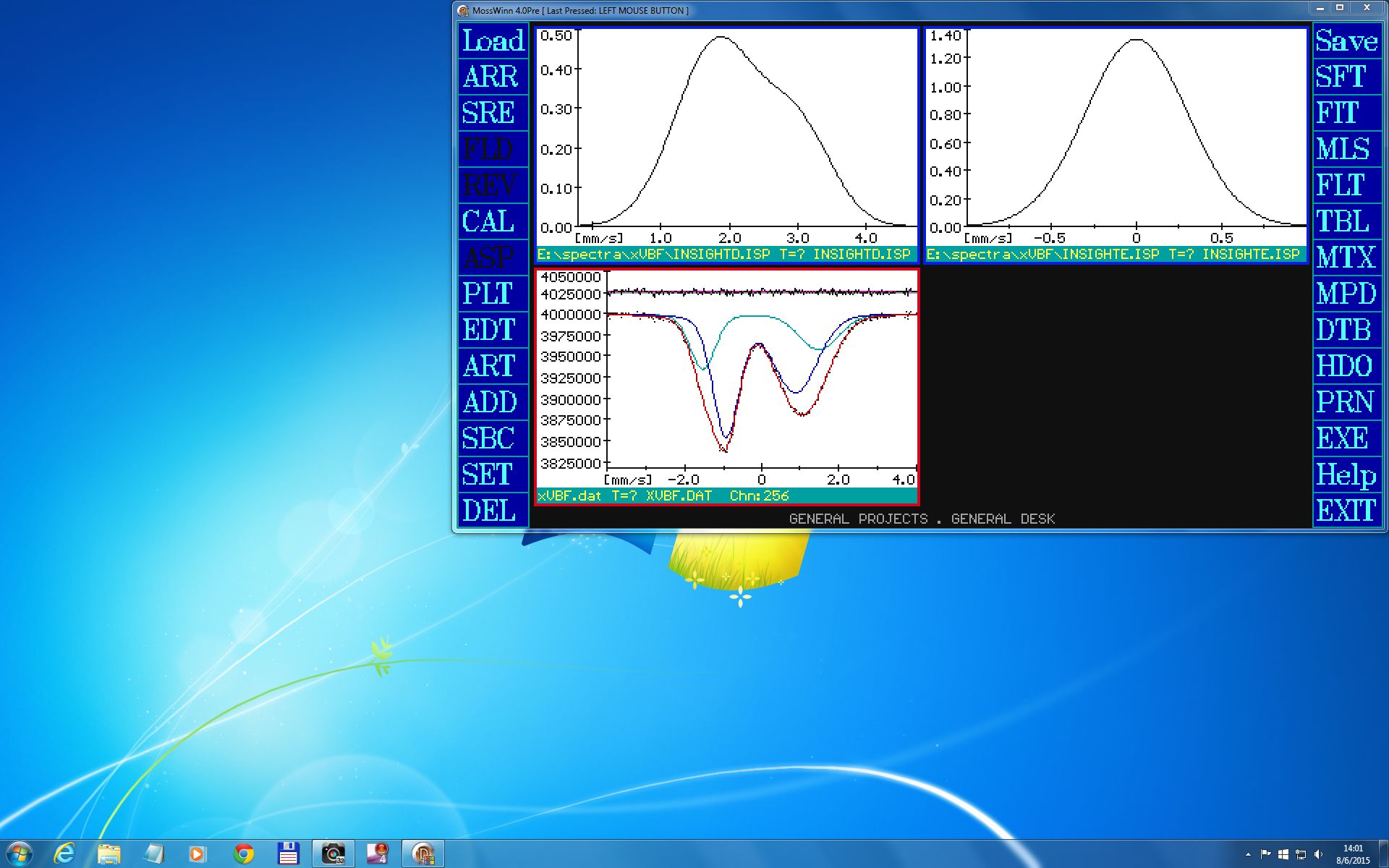
- This example shows how to set up in MossWinn the xVBF (extended Voigt-based fitting) fit model described by the first column of Table 1 in the paper NIM B 129 (1997) 266. Also it is shown how to visualize the cumulative VBF/xVBF distribution curves in MossWinn, and how to export these distributions from the program in the form of ASCII data.
|
 Without narration |
|
|
- This short high-resolution video takes the spectrum and distribution files of the previous example, and shows how to copy the image of all of these data files at once to the clipboard of Windows, and what kind of image is created by MossWinn when choosing this option.
|
 Without narration |
|
|
- This high-resolution video presents a simple example of fitting spectra simultaneously with shared parameters. In this example two 57Fe Mossbauer spectra are fitted simultaneously, each of them to three doublets, by assuming that apart from their relative area fraction corresponding doublets in the two spectra can be described by the same parameters.
The fit proceeds by fitting one of the spectra first, then the second spectrum is added to the fit and the two spectra are fitted simultaneously but with independent parameters, which step is followed by sharing parameters (i.e. constraining corresponding parameters to be equal in the two spectra) gradually with step by step monitoring of the statistical uncertainties to see
how well the applied parameter constraints are justified. The final numerical results are then exported from the program to a document where a table of the results is created.
|
 Without narration |
|
|
- This video presents an 57Fe Paramagnetic Hyperfine Structure (PHS) model spectrum associated with an example taken from the literature.
The model spectrum is described with a PHS model of spin S = 1/2 corresponding to low-spin Fe3+ placed in an external magnetic field of 1300 G being parallel to the γ-ray direction.
The video starts with this model and demonstrates how the various model parameters (such as, for example, the magnitude and direction of the external magnetic field) influence the shape of the model spectrum. It is also shown how to revert the value of fit model parameters to the initial parameter value set previously accepted/saved into the file associated with the spectrum.
(Note that in order to use PHS models in MossWinn, one needs to have either a DBM version license, or a Full range/Select/Lite version license along with a subscription to the MossWinn Services.)
|
 Without narration |
|
|
- This video presents an 57Fe Paramagnetic Hyperfine Structure (PHS) model spectrum associated with an example taken from the literature.
Initially the model spectrum is described with a PHS model of effective spin Seff = 1/2 corresponding to the lowest Kramers doublet of high-spin Fe3+. The video starts with this model and shows how to find a corresponding
model expressed with the real spin value of S = 5/2 along with the associated hyperfine coupling and spin Hamiltonian parameters.
|
 Without narration |
|
|
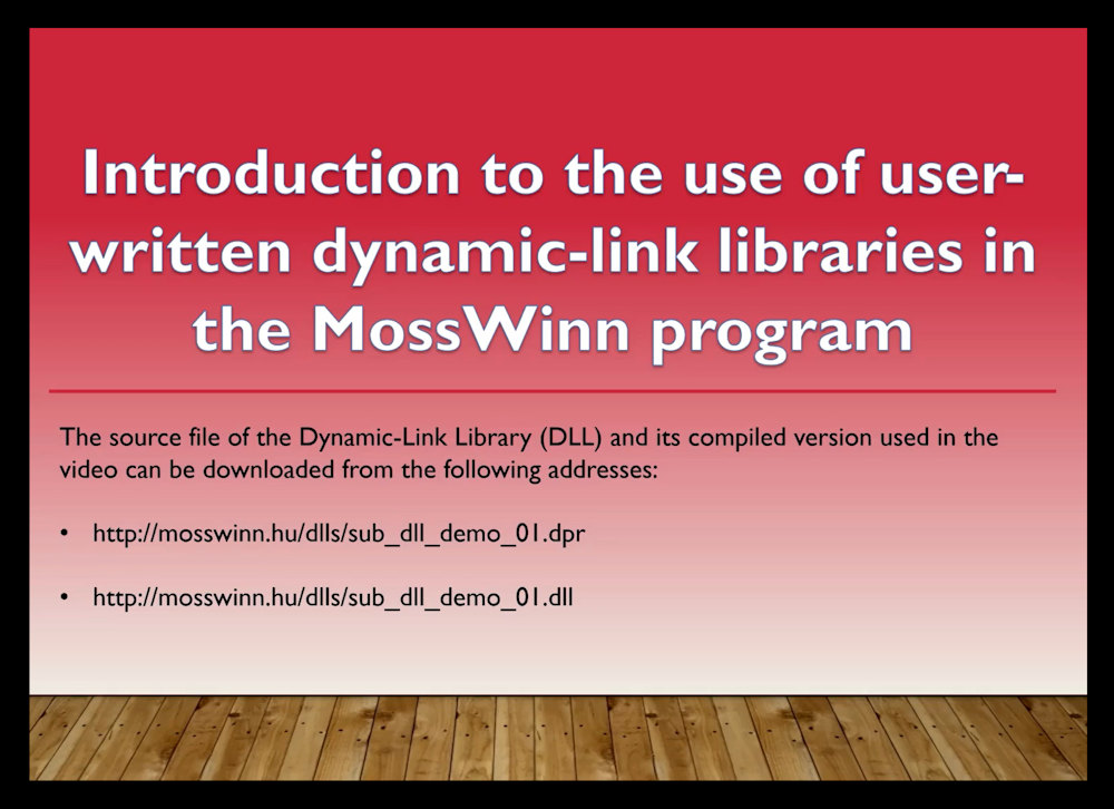
- This video introduces the use of user-written subspectrum-level dynamic-link libraries (DLLs) in the MossWinn program. First it is shown how a DLL library can be compiled via the Delphi 2007 programming environment, then the use of the compiled DLL function is demonstrated with explanations provided regarding the DLL library source code.
The compiled library and its source file are available for download.
|
 English |
|
|
